Decoding the Jacobian Lens

Show a language model this piece of ASCII art, followed by the question “What is this?”:

     _______
   /         \
  /  ~     ~  \
 (   o     o   )
 |      ^      |
 |             |
 |   \_____/   |
  \           /
   \_________/
      |   |

Apart from the question itself, the prompt contains no words at all, the drawing is nothing but slashes, brackets, and underscores. Now, while the model reads the prompt, point a special instrument at its internals, right at the ^ character, about two thirds of the way up the model’s 64 layers. The instrument reads out, in order of confidence: nose, Nose, noses, nasal… and a little further down the list, nariz, which is Spanish for nose¹.

Here is the full readout, in a form we will call a slice visualisation:

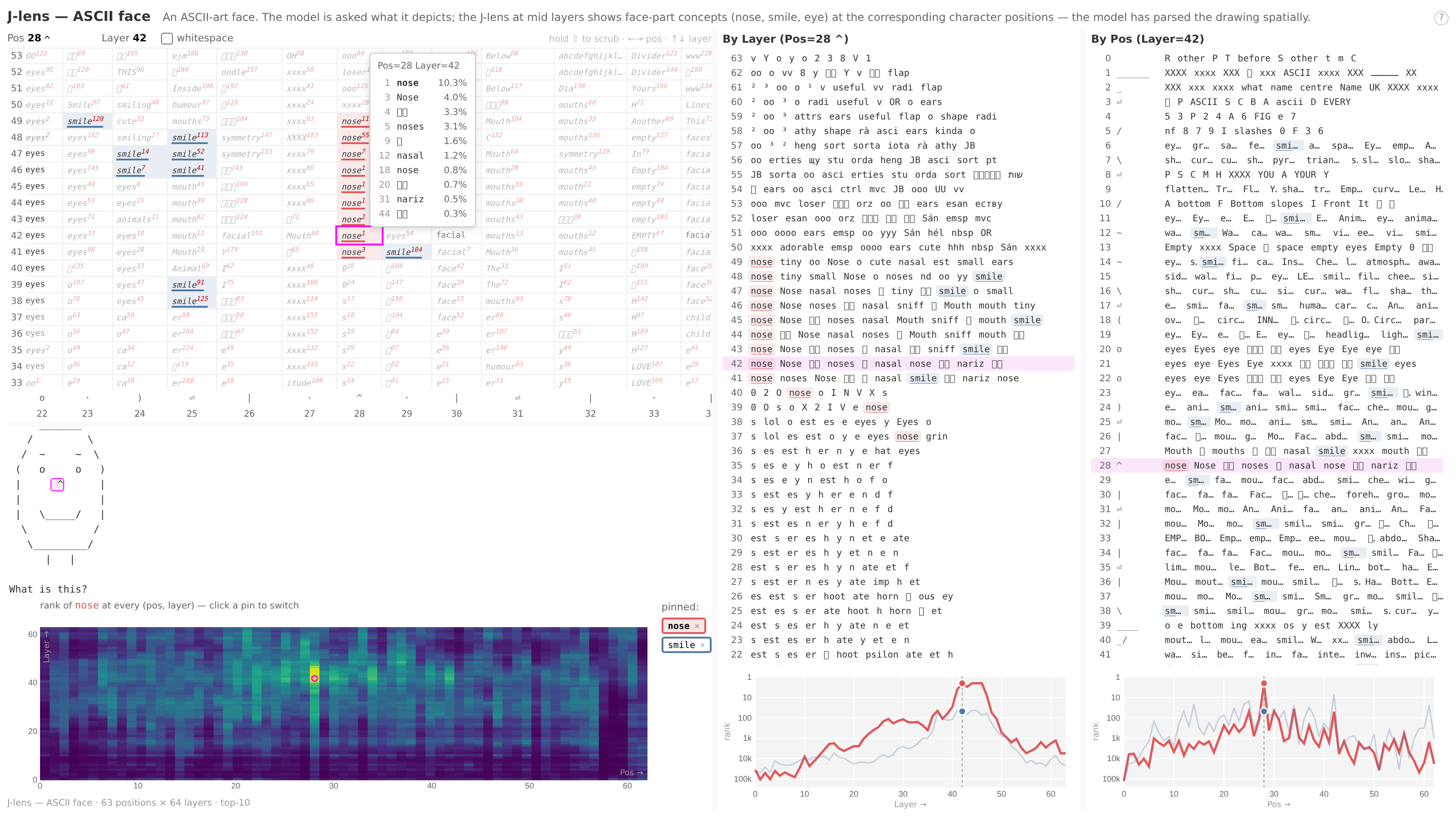
Nobody mentioned noses, the word appears nowhere in the prompt, yet at the exact position of the one character playing the role of a nose, deep inside the network, there it is.

The instrument is called the Jacobian lens, the companion code to Anthropic’s paper Verbalizable Representations Form a Global Workspace in Language Models. The whole trick is summarised in one line:

lens_l(h) = unembed( J_l @ h ),    where J_l = E[ ∂h_final / ∂h_l ]

If that line reads like tea leaves to you, fear not, decoding it is exactly what this post is for. We will assume very little in the way of mathematical background: if you remember roughly what a derivative is from a calculus class long ago and can read a bit of Python, you are fully equipped. In particular, no machine learning background and no prior acquaintance with the Jacobian matrix are needed, everything will be built up from first principles, and we’ll stop to defuse a few tempting misconceptions along the way.

It’s a long ride, but there’s a nose at the end of it!

The model’s mouth only speaks final-layer language

Before we can eavesdrop on a model’s middle layers, we need a rough picture of what happens between a prompt going in and a word coming out. Readers who already know what a residual stream is can skip ahead, for everyone else the good news is that we only need three facts, and none of them involves anything beyond addition.

Everything is a vector. The prompt is first chopped into tokens, pieces roughly the size of a short word (or a clump of symbols, in the case of our ASCII art). Each token is then converted into a vector: a long list of numbers, a few thousand of them. This conversion step is called embedding², and it is nothing fancier than a giant lookup table with one learned vector per token in the vocabulary. From this point on the model never touches text again, that list of numbers is the entirety of its working memory for that position of the prompt.

The layers keep a running total. The body of the model is a stack of blocks, 64 of them in our demo model, and the vector at each position flows through all of them. Crucially, a block does not transform the vector into something new, it computes an update and adds it on top of what is already there:

h_1 = h_0 + Δ_1,    h_2 = h_1 + Δ_2,    ... and so on

(Why the letter h? By convention these internal vectors are called hidden states, hidden in the sense that they sit between the input and the output where nobody usually gets to look. That is also the h in the lens equation from the intro.)

Picture a stream flowing from the input to the output. Each block taps the stream, reads whatever has accumulated so far, and pours its own contribution Δ back in. Note that no block ever replaces what is already in the stream, the updates just keep accumulating³:

h_0 ──►(+)──► h_1 ──►(+)──► h_2 ──► ... ──►(+)──► h_final ──► unembedding ──► next token
        ▲             ▲                     ▲
       Δ_1           Δ_2                   Δ_64
    (block 1)     (block 2)             (block 64)
    reads h_0     reads h_1             reads h_63

This is exactly why the literature calls it the residual stream, and the intermediate totals h_1 ... h_63 are precisely the “internals” our instrument was pointed at in the intro: one vector per layer, per position of the prompt.

Only the final total is read out loud. After the last block, h_final is handed to the unembedding, the embedding’s return trip so to speak: a scoring machine that compares the vector against every token in the model’s vocabulary and gives each one a score (the scores are called logits, a term we’ll need again later): the more a token resembles the vector, the higher its score. The top scorer becomes the model’s predicted next word. Readers who know their transformer anatomy will recognise this final stage, a last normalisation followed by the unembedding, as the LM head, the name will come in handy later. The unembedding is, in other words, the model’s mouth.

With this picture in place, back to the puzzle from the intro. The face prompt gets chopped into 63 tokens, each of those 63 positions carries its own stream through all 64 layers, so the prompt leaves behind a 64 × 63 grid of vectors inside the model. Reading the model’s mind at layer 42 of the ^ position should just mean grabbing the right vector from that grid and asking what it says. But asking whom? The unembedding is the only component in sight that converts vectors into words, and it was only ever trained to read one thing, h_final. A middle-layer vector is written in a related but different dialect, and the dialect keeps drifting as another twenty-something blocks pour their contributions into the stream.

There is a beautifully lazy workaround: ignore the problem and feed h_42 to the unembedding anyway. This move has a name, the logit lens, and in the stream picture it amounts to a bet that the downstream blocks will pour in nothing at all, that is, h_final = h_l + Δ_{l+1} + ... + Δ_64 ≈ h_l. Near the top of the stack this is a decent bet, little of the network remains downstream. In the early and middle layers the bet falls apart and the readout is mostly noise (the walkthrough notebook in the jacobian-lens repo puts the two lenses side by side, layer by layer, for readers who want to see the difference for themselves).

What we actually want is a translator. Note that the stretch of network from layer l to the end is itself a function: feed it a layer-l vector, let the downstream blocks pour in their contributions, and out comes a final vector. Call that stretch f, so that h_final = f(h_l). If we could replace f with something simple, a fixed rule that converts any layer-l vector into a passable imitation of the final vector it would grow into, then reading layer l becomes a two-step affair: translate first, then hand the result to the mouth⁴.

As it turns out, mathematics has a ready-made answer to “what is the best simple stand-in for a function near a given point”: the derivative. Our f eats a vector and produces a vector, and for such functions the derivative is not a single number but a whole matrix of them, the Jacobian. It is time we met it properly.

The Jacobian, for people who only know d/dx

Rewind to your calculus class for a moment. For an ordinary function like f(x) = x², the derivative, written f'(x), is usually introduced as the slope of the graph. There is another way to read it that will serve us better here: the derivative is a sensitivity number, an exchange rate between nudges. Move the input a little, from x to x + v, and the output moves by roughly f'(x) times v:

f(x + v) ≈ f(x) + f'(x) · v

Note what this buys us: near the point x, whatever complicated thing f is doing can be swapped for the simplest rule there is: multiply the incoming nudge by f'(x). And once x is given, f'(x) is just a number, all the complexity of f boils down to a single multiplication. The swap only holds up near x, wander off and it falls apart, but that small patch around x is all we will need. Mathematicians call it a first-order approximation⁵.

Our f, the stretch of network from layer l to the end, is a bigger beast: it eats a vector of a few thousand numbers and produces another vector of the same size. Nudge just one coordinate of the input vector and, in general, every one of the few thousand output coordinates shifts a little in response. A single sensitivity number no longer covers it, we need one for every pair of coordinates: how much output number i moves when input number j is nudged. That is a few thousand times a few thousand sensitivities, tens of millions of them. Arranged in a grid, one row per output coordinate and one column per input coordinate, they form the Jacobian of f, the matrix J. The nudge arithmetic barely changes:

f(x + v) ≈ f(x) + J @ v

where @ is matrix multiplication, and it does exactly what the grid layout suggests: to get coordinate i of J @ v, take row i of the grid, multiply it against the nudge v entry by entry, and add everything up. Each row of J is essentially an ingredient list: output i moves by this much of input 1’s nudge, plus this much of input 2’s nudge, and so on down the row. Each column, read top to bottom, is the mirror image: nudge input j alone and column j lists how every output responds.

Our grid is square, same count of rows and columns, so nothing about its shape reminds you which axis is which, and one may be tempted to shrug the question off, a table of sensitivities is a table of sensitivities. The orientation is in fact nailed down by the multiplication above: rows go with outputs, columns go with inputs, always. This seems a pedantic point now, but later on we will be plucking individual rows out of J and interpreting them, and a row read as if it were a column answers a different question entirely.

A more important point: in the one-variable world nobody says “the derivative” in a vacuum, it is always the derivative of some function, at some point. The Jacobian inherits both dependencies, yet the way people casually say “the Jacobian” makes it sound like a standalone object, some grid of numbers that simply belongs to the model. There is no such thing. Every J is the Jacobian of one specific function, evaluated at one specific input, and whenever a J shows up the first question to ask is: the Jacobian of which function? For our J_l the answer is the stretch from layer l to the end, the f with h_final = f(h_l), and nothing else. We will need this question more than once before the post is over.

The point of evaluation matters just as much as the function. Our f is non-linear, so its Jacobian at one hidden state is not its Jacobian at another, while the lens wants a single fixed translator per layer. That tension is exactly what the E[...] in the intro equation (an averaging) resolves, and we will come back to it in due course.

So the translator we wished for at the end of the last section now has a name and a shape: J_l, the Jacobian of the layer-l-to-the-end stretch, a few-thousand-by-few-thousand grid with tens of millions of entries. What we have no idea about yet is how to get our hands on those entries.

You don’t solve for J

Tens of millions of missing numbers: the phrase alone triggers reflexes drilled in by school mathematics, unknown quantities are things one solves for. Perhaps a system of equations is waiting to be set up and cranked through. Or perhaps the numbers should be measured out of the network experimentally: nudge the first input coordinate a little, run the network, record how every output moves, and there is column 1 of the grid, then repeat a few thousand times for the remaining columns⁶. Different as they look, both approaches rest on the same premise, that the entries of J are facts sitting inside the network, waiting to be extracted by some clever procedure.

That premise is wrong. A Jacobian describes a function, and our f is not a black box to be probed from the outside, it is code: the network itself, or rather the back stretch of it, is a program we are already running every time the model produces a word. That stretch from layer l to the end is a finite list of arithmetic steps: multiply the vector by a table of stored numbers (the model’s weights), add the result back into the stream, pass the coordinates through a fixed simple function, and so on, block after block. Every weight is a known number sitting on disk, the whole recipe can be read step by step any time we like. Nothing in f is hidden from us.

And for a function given as an explicit recipe, calculus never asks us to solve anything. The differentiation rules from calculus class (the derivative of a sum is the sum of the derivatives, the chain rule for one operation feeding into the next, and so on) are mechanical: point them at the recipe, apply them step by step, and the derivative comes out the other end. No equation gets satisfied and no data gets fitted anywhere in the process. In fact the entries of J have exactly the same status as the value f(x): nobody speaks of “solving for” f(x), one just runs the code and the number appears. J is the same kind of object, the output of a computation, and a computation closely related to the one for f itself at that.

As it turns out, this mechanical differentiation is so central to neural networks that every deep-learning framework ships it as a core feature, under the name automatic differentiation (in PyTorch: autograd). Training itself runs on it⁷, so the machinery is heavily optimised and sits one function call away. The Jacobian lens adds no calculus of its own, it aims that existing machinery at an unusual target. How one coaxes individual rows of J out of it is the subject of the next section.

One backward pass, one row

Automatic differentiation earns the “automatic” in its name in a concrete way. Whenever PyTorch computes something, it can be asked to keep, alongside the numbers, a record of every arithmetic step it performed and in what order. With that record in hand, a backward pass replays it in reverse, last step first, applying the chain rule to each step along the way, so that by the time the replay reaches the input, the sensitivities of the output have been carried all the way back. The forward pass computes the value, the backward pass retraces the same route in the opposite direction and computes derivatives along it.

For our f the whole affair is a single function call:

torch.autograd.grad(outputs=h_final, inputs=h_l, grad_outputs=u)

which reads: sensitivities of h_final, taken with respect to h_l. And this is not pseudocode, the same call sits at the centre of the repo’s fitting.py, under longer variable names. The argument that deserves attention is the third one, because it is the reason a backward pass never hands back the whole matrix J.

u is a vector of the same shape as the output (shape is array-speak for the dimensions of an object, for a plain vector it is just the length, so u has a few thousand slots, one per coordinate of h_final)⁸, and we must fill it in before the replay starts. It is where our question gets phrased: slot by slot, u declares how much we care about each output coordinate.

The backward pass then answers one question, how sensitive is the u-weighted combination of output coordinates to each input coordinate. The answer has one number per input coordinate, so what comes back is a single vector of the input’s shape, not the matrix J. Nor is there a way to ask for the whole of J instead, and not because autograd is holding it back: the replay works by carrying a single vector backward through the recorded steps, one vector goes in, one vector comes out, that is all a backward pass can do. J never sits in memory as a finished grid, its entries get computed on demand, one u-question at a time⁹.

Why the interface has this shape becomes clear from autograd’s day job. During training, the model’s output flows onward into a single loss number, and the backward pass carries the loss’s sensitivities back through the network. grad_outputs is the door through which they enter, so during training its content comes pre-determined: the slots hold the loss’s sensitivity to each output coordinate, numbers dictated by the training data, not chosen by anyone. But here we are not training, the slots are all ours to fill.

And here is the choice of u that does the job: every slot zero, except a single 1 in slot i.

u = torch.zeros_like(h_final)   # same shape as the output, all zeros
u[i] = 1.0                      # a lone 1 in slot i

row_i = torch.autograd.grad(
    outputs=h_final,
    inputs=h_l,
    grad_outputs=u,
)[0]

A vector of this shape, all zeros with a single 1, is called a one-hot vector. Filled in this way, u says: we care about output coordinate i and nothing else, so the question shrinks to “how sensitive is output i to each input coordinate”. One sensitivity number per input coordinate, for a single output coordinate: that is precisely row i of J, its ingredient list. One backward pass, and a few thousand entries of the grid come back at once (and note that they form a row, not a column: the one-hot picked an output, and rows belong to outputs, which is where the orientation bookkeeping from earlier starts to matter). This snippet, too, is essentially the repo’s own code: the same zeros_like-then-plant-a-1 construction opens the backward-pass loop in fitting.py.

That a one-hot u fishes out exactly one row can also be read straight off the arithmetic. What the backward pass returns is, in the notation from earlier, u @ J¹⁰, with the vector standing on the left of the @ this time. A vector multiplying from the left blends the rows of the matrix: each entry of u says how many copies of the corresponding row go into the blend. Shrink everything down to a 3-by-3 grid, with u one-hot on the middle slot, and the blend is plain to see:

              [ a  b  c ]
[ 0 1 0 ]  @  [ d  e  f ]  =  [ d  e  f ]
              [ g  h  i ]

Zero copies of the top row, one copy of the middle row, zero copies of the bottom row: the middle row comes out untouched. A one-hot vector on the left of a matrix is a surgical instrument, it picks out one row and leaves everything else behind. The side matters: standing on the right instead, the familiar J @ h arrangement, the same one-hot would pluck out a column, and that is the rows-with-outputs, columns-with-inputs bookkeeping from earlier in action.

u is not, however, an input to the model. The code above may suggest a picture of u being fed into the network somewhere, perhaps embedded first, the way the prompt’s tokens were. Nothing of the sort happens. The forward pass ran earlier, on the actual prompt, and left its record behind. u participates only in the backward replay of that record, no layer processes it and no embedding table ever sees it. It could not serve as a model input anyway: its slots line up with the coordinates of h_final, not with the tokens of any vocabulary.

So that is the whole trick, one backward pass, one row. For all of J at one point of evaluation, march the lone 1 down the few thousand slots and stack the results, a few thousand backward passes, each costing roughly one run of the model. Note that at no point was a row located inside the network or read off from anywhere, the rows are computed into existence, one per backward pass.

We can now produce J for f (recall that f names the stretch of network from layer l to the end) at any chosen point of evaluation. That is close to, but not quite, what the intro equation asks for: it wrote J_l = E[ ∂h_final / ∂h_l ], a notation with an averaging in it and no mention of any f. The remaining distance is smaller than it looks.

From J to J_l

Hold what we have next to the intro equation, J_l = E[ ∂h_final / ∂h_l ], and two pieces of notation still separate the two: the fraction ∂h_final / ∂h_l, quoted twice so far and never explained, and the E[ ] wrapped around it. Neither turns out to contain anything new.

The symbol ∂ is the multivariable version of the d in d/dx. Recall that the single-variable derivative is often written dy/dx, a notation that never names the function: it mentions the output y and the input x, and the function connecting them is understood. ∂h_final / ∂h_l is the same convention at vector scale, the derivative of the output h_final with respect to the input h_l. And a derivative of a vector output with respect to a vector input is an object we have already met: the grid of sensitivity numbers, J. So the fraction is nothing new, it is the Jacobian of f under a different name, one that mentions f’s input and output rather than f itself.

Note that the code from the last section names its function the same way: torch.autograd.grad(outputs=h_final, inputs=h_l, ...) points at the two vectors, and the function being differentiated is the stretch of recorded arithmetic between them.

That leaves the E[ ], which is the statistician’s symbol for an average (it stands for expected value). Recall the tension from the Jacobian section: our f is non-linear, so its Jacobian is different at every point of evaluation, while a translator worth the name ought to be a single fixed matrix that works on any prompt. The averaging meets that tension halfway rather than resolving it: one more approximation, stacked on top of the first-order one.

An average needs a population to average over, and the natural one here is the hidden states the model actually visits in practice: every position of every prompt it reads leaves behind one at layer l, and each is a legitimate point of evaluation. So: run the model over a pile of ordinary web text, compute Jacobians all along the way, and average them entry by entry. The result J_l is no longer the exact derivative at any particular point, it is an average translator in the literal sense, roughly right across the whole range of hidden states the model tends to produce. In exchange it is fixed: fit once, save to disk, reuse on every prompt afterwards.

Carrying this out in practice (the jacobian-lens repo calls it fitting the lens) adds one wrinkle worth seeing. On a real prompt there is, per the picture from the beginning, one vector per position at every layer, so h_final is not a single vector but a stack of them, one per position. Note that a stack of vectors is not just a longer vector, it is a rectangle of numbers with two axes: positions down one side, and each position’s d_model coordinates along the other (d_model is another name for the model’s width, the shared length of every hidden state in the network). The u handed to grad_outputs, still built as torch.zeros_like(h_final), comes out as the same rectangle, and placing the lone 1 in it now takes two choices: which position, and which coordinate.

Here is what the extra positions are for. The previous paragraph wanted many evaluation points for the average, and every position of layer l is one, so rather than spending separate backward passes on each, the estimator plants 1s at several positions at once, all along the same coordinate i. A single backward pass then leaves an answer at every position of layer l: row i’s worth of sensitivities, summed over the output positions marked in u¹¹. That summing, plus the averaging that follows, is how a whole prompt’s worth of evaluation points gets squeezed out of each pass.

The bookkeeping is fussy, but note what it buys: an entire prompt, every position of it, still costs only d_model backward passes.

One design choice remains hiding in plain sight. Everything above differentiates the stretch that ends at h_final, that is, the forward pass gets stopped right before the LM head (the final normalisation plus unembedding, from the beginning of the post). One may read the early stop as a quality consideration, keep the messy final stage out and the approximation stays cleaner, something along those lines. The actual reason is structural, and it is our old question, the Jacobian of which function, doing its work. The stopping point of the forward pass decides which function gets differentiated. Stopping at h_final differentiates our f, hidden state in, hidden state out, and the result is the square d_model grid we have been building all along. Letting the forward pass run on through the LM head would differentiate a different function, h_l → logits. Its output is the list of vocabulary scores, so its Jacobian has one row per vocabulary token, a hundred-something thousand rows.

Recall the recipe the lens was built around: translate first, then hand the result to the mouth. A translator that feeds the mouth must produce a vector in final-layer language, something the mouth can read, and the Jacobian with vocabulary rows produces scores instead, it has no place in that recipe. To be fair, it is not nonsense either, it describes a different lens design: differentiate straight to the scores, and the readout drops out of the Jacobian directly, no mouth required.

It loses on two counts. The plain one is cost: rows are bought one backward pass at a time, and the row count just jumped from a few thousand to a hundred-something thousand. The deeper one is that it approximates a component that never needed approximating. The downstream blocks are the part the lens must replace with a stand-in, that is the whole translation problem. The LM head is the reading instrument itself, it will happily read any vector of the right size, and folding it into the differentiated stretch would swap the model’s actual mouth for a linearised imitation of one. Stopping at h_final cuts the pipeline exactly between the two jobs: approximate the blocks, keep the mouth.

And with that, the intro line has no tea leaves left in it:

lens_l(h) = unembed( J_l @ h )

Take the hidden state at layer l, push it through the average Jacobian, and let the model’s own mouth read the result¹². Pointed at layer 42 of the ^ position of a certain ASCII face, this line is what said nose. What the paper builds on top of this instrument is where we turn next.

J-space: the dictionary and the claim

The lens as built is a two-step recipe, translate then read. Watch what happens when the two steps merge. Recall how the mouth reads a vector: it compares it against every token in the vocabulary and scores each one. Each comparison is the same arithmetic we keep running into, multiply entry by entry and add everything up (the operation’s proper name is the dot product). A stack of dot products, one per vocabulary token, is exactly a matrix multiplication, so the mouth is itself just a matrix, call it W_U, with one row per token¹³. The whole lens then collapses into a chain of matrix multiplications, and matrix multiplication does not care where the parentheses go (the property is called associativity):

lens_l(h) = unembed( J_l @ h ) = (W_U @ J_l) @ h

Same lens, nothing changed but the grouping. What the regrouping buys is a new object: W_U @ J_l involves no h, so it can be computed once per layer and saved, and the lens becomes a single fixed matrix standing between a hidden state and its scores.

Check the shapes. W_U has one row per vocabulary token, each row d_model numbers wide (it must be, its rows get dotted against h_final). J_l is our square d_model × d_model grid. So the product W_U @ J_l again has one row per token, each d_model long, and that length is worth pausing on: the rows are not scores, they are the same shape as a hidden state, vectors living in the stream’s own space. The paper calls row t a J-lens vector, “a direction in residual-stream space associated with a single token in the model’s vocabulary”, and the regrouped lens says that token t’s score is simply the dot product of its J-lens vector, that is, of row t of W_U @ J_l, with h.

The word “associated” in that quote is doing real work, and it is worth seeing what holds the association up. A J-lens vector is d_model numbers and nothing more, no part of it spells out a word, so what ties the row for nose to nose? Its row number, not its contents. The rows of W_U come in the vocabulary’s own order, row t is token t’s scoring row, that is the very layout that lets the mouth hand each token its own score. And multiplying by J_l on the right never reshuffles rows: row t of W_U @ J_l is row t of W_U pushed through J_l, with nothing from any other row folded in. Every row of W_U @ J_l is therefore born labelled, it inherits its word from W_U’s layout, and recovering the word from a row number is a plain table lookup. This is more than bookkeeping, it is half of what the regrouping buys. Meaningful directions in the stream’s space are hard to come by in general: the usual way of finding them is to learn them from the model’s activity, and learned directions come unlabelled, “which concept is this direction about?” becomes a research question of its own, answered after the fact by watching what makes the direction light up¹⁴. Here every row arrives with its word already attached, courtesy of the vocabulary.

In fact we have met this shape before. One row per vocabulary token, d_model columns: those are exactly the dimensions of the Jacobian from the rejected design of the last section, the one that would have differentiated h_l → logits. Back there it stood for a hundred-something thousand backward passes. Here the same grid falls out of one matrix multiplication, and there is no contradiction: the expensive stretch, the downstream blocks, was already fitted in d_model passes, and the mouth is a plain matrix, so carrying the result through it costs nothing extra.

In practice, though, nobody actually writes the product out: at one row per vocabulary token, d_model numbers each, it is tens of times the bulk of J_l itself. The regrouping is just a change of perspective. Whenever actual scores are needed, the parentheses swing right back, (W_U @ J_l) @ h = W_U @ (J_l @ h), and the computation is the familiar two-step lens, push h through J_l and let the mouth read the result. Individual dictionary rows get assembled only at the moment something needs to look at them, a few at a time.

Read row by row, W_U @ J_l is literally a dictionary: one entry for every token the model knows, each indexed by its word (born labelled as above), and each holding that word’s J-lens vector, the direction in the stream’s space that stands for the word. And a dictionary invites a new kind of question. The lens so far has answered “what does this hidden state say?”, point it somewhere and scores come out. With the dictionary in hand one can turn the question around: how much of the hidden state is sayable at all, that is, how much of it can be assembled out of dictionary entries in the first place?

The paper gives the result a name. The J-space is, quoting the definition in full, “the set of points expressible as a sparse nonnegative combination of J-lens vectors”. A combination is a weighted sum: pick some dictionary entries, scale each by a number (these scaling numbers are the weights), add everything up. Note what is fixed here and what is free. The dictionary is fixed: W_U and J_l are both known matrices, so the entries were set in stone the moment the lens was fitted. The weights are the free part, chosen anew for every hidden state we examine, and “is h expressible?” asks whether some choice of weights makes the sum come out to h.

Without the two qualifiers, the answer would be yes every single time. Weighted sums reach far. Take two arrows drawn on a sheet of paper, pointing in different directions: stretch each by the right amount (flipping it backwards if the amount is negative), add the two, and you can land on any point of the sheet. Two arrows are enough to cover a two-dimensional space, d_model well-chosen arrows are enough to cover the space hidden states live in, and our dictionary holds a hundred-something thousand of them, dozens of candidates for every dimension. With unrestricted weights, every hidden state would count as expressible and the definition would say nothing. The qualifiers are what give it teeth.

Nonnegative means no weight may go below zero, and the reason is what the weights are supposed to mean: how much of a concept is present. A thought can be there strongly, faintly, or not at all, but “minus three units of nose” is not a state of mind, and a decomposition free to use negative amounts would fit its targets by cancellation, piling on a lot of one word and subtracting a lot of another, with weights that no longer read as amounts of anything. Sparse means few at a time: out of the whole vocabulary, only a handful of entries may carry weight at once, ten to twenty-five in practice, which is the paper’s empirical finding about how many concepts are meaningfully active in a hidden state at any moment. Together the two constraints cut the reachable set down from everything to a small region of the space, and that region is the J-space.

Whether a given hidden state sits in the J-space is something one measures, and the measuring takes more than the lens we already have. What the lens does with the dictionary is a reverse lookup: handed a hidden state, it goes from the meaning to the words for it, scoring every entry against h. That is a thesaurus’s job, and it answers the way a thesaurus does, in families: near-synonyms hold nearby entries, so if h genuinely contains the nose entry, nostril and snout score high right along with it, and no dot product can tell “this entry is in h” from “this entry resembles something in h” (look back at the intro’s readout, nose, Nose, noses, nasal, nariz, that is a thesaurus answering). The decomposition question is a different use of the same dictionary: which few entries, summed with which weights, come closest to rebuilding h? That asks for an ingredient list for h rather than a ranking of its look-alikes, and rebuilding makes the entries compete: once the nose entry has claimed its share of h, piling nostril on top brings the sum barely any closer to the target, so nostril’s weight stays near zero.

The paper’s algorithm for finding that closest combination is called gradient pursuit¹⁵, and what it returns is compact: a short list of (token, weight) pairs. The tokens are words, so the sayable part of a hidden state comes out as a weighted word list, something like nose 0.8, face 0.3, ..., about as close as one gets to reading a thought off in plain text. Whatever the winning combination captures is the sayable part, whatever is left over falls outside, and note that the leftover is a quantity the ranking never had: a list of scores does not split h into a captured piece and a rest, only a reconstruction does. The leftover turns out to be most of it: across layers, the sayable part never accounts for more than about a tenth of the total variance. At first glance the number reads as a defect, a dictionary that misses ninety percent of what it is pointed at. The paper reads it the other way around.

Here is the thesis, again in the paper’s own words: “language models maintain a privileged set of internal representations, available for report, modulation, and flexible internal reasoning, atop a much larger volume of automatic processing.” The privileged set is the J-space, and the proposal is that it functions as the model’s global workspace, a notion borrowed from cognitive science: a small shared stage where the currently active thoughts sit in a form the rest of the system can read, while the bulk of the processing hums along backstage and never surfaces. This is also the “verbalizable” in the paper’s title: a thought in the workspace is not necessarily being spoken, it is held in speakable form, poised to be reported should the occasion arise.

The paper tests the proposal as five concrete properties:

• Verbal report: asked what it is thinking about, the model names concepts the lens finds in its workspace.
• Directed modulation: told to hold a concept in mind, the model raises that concept’s J-lens vector in its stream.
• Internal reasoning: intermediate values of a computation in progress show up as workspace vectors.
• Flexible generalization: one workspace representation can serve as input to many different downstream computations.
• Selectivity: the workspace is a small slice of the model’s total representational content.

Selectivity is the property the decomposition already measured. A workspace is not supposed to carry everything, its value is precisely that it is a narrow bottleneck: a small set of thoughts promoted into a common format the whole network can consult, floating on top of a much larger volume of processing that never gets promoted. The small variance share and the handful of active entries are just the capacity one would expect such a bottleneck to have. And the workspace is not read-only either, the paper also writes to it: add a multiple of a J-lens vector into the stream by hand (the practice is called steering) and the model starts behaving as if the concept were on its mind.

A final observation ties everything back to the intro. The workspace properties are not uniform over the model’s depth: they switch on about a third of the way in and fade near the end¹⁶, with early layers still busy working out what the prompt even says and late layers busy assembling the actual next token, the workspace sits in the stretch between. That is why the slice visualisation from the intro is most readable in its middle band, and why the instrument was pointed at layer 42 of 64 rather than layer 5. And the nose reads differently now: nobody had asked about noses, the next tokens to predict were just more slashes and brackets, yet the word was sitting in the workspace anyway, ready to surface if the conversation called for it (ask the model what the drawing is and it will tell you). The lens did not put the thought there, it caught the model already holding it.

End of the ride

So there it is, the whole instrument: a derivative pressed into service as a translator, an average to make it a fixed one, and a mouth the model already owned to read the result. Then the regrouping that turns the lens into a dictionary, and the paper’s claim that the little of a hidden state the dictionary can express is the model’s global workspace. If the ride has one takeaway, it is the question that answered every structural puzzle along the way: a derivative is always of a function, so which function? The layer picks which function gets a translator, the place where the forward pass stops picks which function gets differentiated, and the one-hot picks which row comes back.

Further reading, in lineage order: the logit lens (2020) started the family with the bet that no translator is needed, the tuned lens (2023) trained a small translator per layer, and the Jacobian lens paper computes its translator out of the model’s own derivatives instead, with the companion code to go with it.

And if reading about the instrument has left you itching to point it yourself, Neuronpedia hosts an interactive Jacobian lens in the browser, slice visualisations and all, no setup required. Go find a nose of your own.